Genotyping Cyclospora: from haplotype calls to outbreak clusters

Anton Nekrutenko¹ and Sergei Kosakovsky Pond²

¹ Dept. of Biochemistry and Molecular Biology, The Pennsylvania State University, University Park, PA, USA
² Dept. of Biology, Temple University, Philadelphia, PA, USA

This is the second post in a series on the analysis of Cyclospora (taxid 44417) outbreaks. Part 1 described the parasite, the assay, the public sequencing record and the 203-specimen benchmark. This part describes what CDC's typing pipeline does with a haplotype sheet, what happens when the published code is run, and how an open reimplementation turns the same sheet into clusters. Part 3 reports the four-arm benchmark these pieces were assembled into.

Everything here uses the benchmark defined in Part 1: 203 clinical specimens from BioProject PRJNA578931 [19], labelled by two epidemiologically-defined 2018 outbreaks—Vendor A (salads, 99 specimens) and Vendor B (vegetable trays, 104) [4]—taken from REFERENCE_CLUSTER_LIST/2018_gold_clusters.txt in CDC's typing repository [6]. Those labels come from food-exposure investigation and are independent of any sequence data. 153 of the 203 appear in CDC's deposited haplotype sheet [8], 98 Vendor A and 55 Vendor B, and that is the set most numbers below are computed on. Every denominator is stated, because they differ.

What CDC's typing workflow does

The published workflow consists of three modules [6] executed sequentially.

Module 1—Consumes sequence reads and produces a haplotype list

MODULE_1_hap_caller.sh turns paired FASTQ into presence calls, one specimen at a time [6]:

Trim. BBDuk removes Illumina adapters, right-trimming with k=23 mink=11 hdist=1 and discarding anything below 50 bp. The four audit documents discussed later in this post [12] describe this step as cutadapt, which the caller invokes only inside the junction module.
Merge. bbmerge-auto merges the read pairs. The PARTs are 67–122 bp and the reads are 2×250, so a merged pair covers a whole haplotype window with room to spare.
Collapse. CD-HIT-est clusters the merged reads at -c 1, which is 100% identity, not the 99% those documents state. Identical reads become one representative with a count.
Name. Each distinct sequence is looked up in a dictionary of already-named haplotypes. The lookup is blastn at -perc_identity 100 -qcov_hsp_perc 100 -word_size 7 -dust no: the match must be exact and full-length, so this is a lookup, not a similarity search. A sequence that matches takes that entry's name. One that matches nothing stays unnamed — whether it ever earns a name is decided separately and far more strictly, in the next section.
Decide what counts as present. Having a name is not the same as being reported. A named haplotype enters the specimen's row only if its read count clears two thresholds at once: a fixed floor (DEPTH_FOR_CALLING, 20) and a moving one at 10% of that specimen's mean coverage at that locus. The second usually binds: median mean per-PART depth here is 5,927× for Vendor B and 10,021× for Vendor A, putting the 10% threshold at 590–1,000 reads — thirty to fifty times the fixed floor.
The junction separately. Mt-Junction is a variable-copy repeat array and is not typed by alignment. Reads are converted with MIRA 4.0.2, assembled with CAP3, trimmed against the flanking motifs with cutadapt, and matched to the twenty junction reference sequences [9].

The output is the haplotype detection sheet: one row per specimen, one column per named haplotype, X where detected. A real corner of the benchmark sheet — four specimens and the six columns they populate across two loci [8]:

`Seq_ID`	378·D Hap2	378·D Hap4	378·D Hap7	378·D Hap9	CDS1·A Hap1	CDS1·A Hap2
`C_IA031_18`		X	X	X
`C_IA013_18`	X	X
`C_IA062_18`			X			X
`C_IA059_18`					X

A specimen can carry several haplotypes at one locus. C_IA031_18 has three at Nu_378_PART_D. That is not an error but a mixed infection, and 130 of the 153 benchmark specimens carry more than one haplotype there. Any distance must therefore compare sets of alleles, not single values — which is why the next section's methods look as they do.

How a sequence earns a name

The dictionary is a list of haplotype sequences that already have names, like Nu_378_Hap_4. Step 4 is a lookup against it.

Many sequences will not be there, for two very different reasons: the specimen carries a variant nobody has catalogued, or the sequence is an artefact — a sequencing error, a PCR slip. At 5,000–10,000× an error does not look like noise. The same mistake recurs across hundreds of reads and arrives looking clean and entirely plausible. Frequency alone cannot separate the two.

A separate script, Finding_New_Haps_SNP_Based_Module.sh [6], decides whether an unrecognised sequence earns a permanent place in the dictionary, and it demands far more evidence than an ordinary call:

	to record a specimen as carrying a known haplotype	to mint a brand-new named haplotype
raw reads	20 (`DEPTH_FOR_CALLING`)	100 (`-N`, default 100)
share of that locus's reads	10%	25%

Both must hold, so the stricter governs. Inventing a name costs five times the fixed depth and two and a half times the relative depth of reusing one. The code says so itself: "To write a new haplotype to the reference database, I want it to have at least 100 times coverage AND I want the new haplotype to be supported by at least 25% of the reads for that locus (whichever value is higher will be the final cutoff used)."

The gap exists because of how far a mistake travels. A wrong call on an existing haplotype is one bad cell in one row. A wrongly minted new haplotype is written to REF_SEQS/BLASTING/NEW_HAPS/ and concatenated back into the dictionary, so every later specimen is compared against a name describing a sequencing error. One mistake becomes a column in every sheet built from then on.

A high bar to invent a word and a low one to reuse it is the right instinct, and the design decision here we would keep. The bookkeeping around it is harder to defend.

The name is a position, not a property. A promotion is named <marker>_Hap_<n+1>, where n is however many that marker happens to have at that moment. The name records arrival order and nothing recoverable from the sequence.

The dictionary is rewritten mid-run, so the pipeline is order-dependent. A promoted sequence can name the next specimen. Something novel at specimen 5 can be an exact match by specimen 60, so the same specimens in a different order can come out with different names, or with a haplotype counted as known in one run and novel in another. Nothing pins the order or records which was used.

The marker comes from a deliberately loose BLAST. Which locus a new haplotype belongs to is decided by re-BLASTing at -perc_identity 75 -qcov_hsp_perc 85 with -max_target_seqs 1. That flag does not mean "best hit" — it means the first hit satisfying the search, an artefact of BLAST's internal ordering rather than a ranking [20]. A misassignment here puts a column under the wrong locus in every sheet built afterwards.

None of this shows in the sheet. By Module 2, Nu_378_Hap_31 and Nu_378_Hap_4 are indistinguishable columns.

Module 2—a haplotype sheet to a distance matrix

MODULE_2_eukaryotyping.sh runs run.r, which computes two distances and combines them [6, 7].

The Barratt heuristic [1] scores every pair of specimens at every locus from the two sets of alleles seen there. An allele here is a named haplotype, the phased sequence variant Part 1 described. At a nuclear locus it computes a penalty for sharing nothing and a smaller one for sharing something, so a pair sharing any allele scores at most 2 there and only a pair sharing nothing scores higher. The next section works the arithmetic through on a real pair.

That penalty is then multiplied by two weights. The first is the Shannon entropy of the allele frequencies at that locus — a number in bits, large when several alleles sit at similar frequencies and near zero when one dominates — meant to give variable loci more influence. The second is a rarity factor from the fraction of the batch carrying the shared alleles, meant to credit a shared rare allele more than a shared common one.

Mitochondrial loci use a separate rule: zero if the two specimens share any allele, 2x if they share none, with no accounting for how many alleles each carries. On this benchmark that rule scores Mt_Cmt, the junction — the locus carrying most of the signal. Loci missing in one specimen are carried as NA and filled by a two-pass imputation before the per-locus scores are averaged.

Worked example — the Barratt heuristic on one real pair

Take the two specimens from the sheet excerpt above, at the locus shown there, Nu_378_PART_D:

C_IA031_18   Hap4  Hap7  Hap9
C_IA013_18   Hap2  Hap4

They share Hap4. Every quantity the heuristic uses comes from those two lists:

symbol	definition	here
`n`	how many alleles the smaller of the two specimens carries	`min(3, 2)` = 2
`x`	the two counts added together — a sum, not a merged set, so a shared allele is counted twice	`3 + 2` = 5
`y`	how many alleles the two specimens have in common	just `Hap4` = 1
`jj`	a per-locus multiplier, fixed at 2 for every locus (see below)	2
`w`	a penalty computed from `n` and `x`, used only when the pair shares nothing	5
`z`	a credit computed from `n`, `x`, `y` and `jj`, used only when the pair shares something	2

w and z are each one line of arithmetic over those counts, and only one is ever used, because a pair either shares an allele or does not:

case	`δ_raw`
the pair shares no allele (`y = 0`)	w
the pair shares at least one (`y > 0`)	2·jj − z

The code picks between the two without an if. It writes both as a single sum and multiplies each by a true/false test, which R evaluates as 1 or 0, so exactly one term survives:

delta_nu_raw = w * (y == 0)  +  2 * jj * (y > 0)  +  <credit term>
#                  ├ 1 if they share nothing      ├ 1 if they share something
#                  └ 0 otherwise                  └ 0 otherwise

Here y = 1, so the first term is multiplied by 0 and vanishes and the second applies:

δ_raw = 2·jj − z = 4 − 2 = 2

The 4 there is not a constant in the source; it is 2 × jj, and jj is defined per locus as

m <<- rep(1, nloci)
jj = 2 * (m[j] == 1) + m[j] * (m[j] > 1)

m has one entry per locus, is set to all ones on line 32, and is never assigned again anywhere in the codebase. So m[j] is always 1, jj is always 2, the share-something ceiling is fixed at 2·jj = 4, and the credit window is fixed at z ∈ {2, 3, 4}. m has the shape of a per-locus tunable — plausibly expected copy number — but ships as a constant, and every "4" below is that constant showing through.

Then the weights. This locus has entropy H = 1.51 bits, carrying four alleles at frequencies 0.50, 0.31, 0.19 and 0.004. The rarity factor asks how special the shared allele is: Hap4 is carried by 138 of the 145 specimens with data, so P = (138/145)² = 0.91 — sharing it is barely evidence of anything, and the weight says so. The locus contributes

δ = H × δ_raw × P = 1.51 × 2 × 0.91 = 2.73

One locus, one pair. The same runs at every locus, and the scores are averaged.

What the arithmetic actually rewards

Running the same code over every configuration that can occur shows the behaviour more clearly than the formulas do:

what the two specimens carry	`x`	`n`	`y`	`δ_raw`
one allele each, the same one	2	1	1	0
two each, sharing both	4	2	2	0
one vs three, sharing the one	4	1	1	1
two each, sharing one	4	2	1	2
three vs two, sharing one	5	2	1	2
one allele each, different	2	1	0	4
two each, sharing none	4	2	0	4
one vs three, sharing none	4	1	0	5

Two features stand out, and both matter later.

Sharing anything caps the score at 2; sharing nothing starts at 4. The two regimes do not overlap. The heuristic is effectively a switch — any allele in common at this locus? — with slight gradation inside each answer.

A mixed infection is rewarded, not penalised. Compare rows 3 and 6: one strain against that same strain plus two others scores 1, while two specimens carrying single different strains score 4. The co-infected pair is treated as four times more similar. Hold onto this, because the audit documents examined later claim the opposite — that this configuration yields "a large penalty δ_raw = 1 + x = 4, falsely excluding Patient B from the outbreak cluster". It does not. That reading takes x for the union of the two allele sets; the code computes the sum, and the share-something case applies regardless.

The Plucinski Bayesian component [3, 7] never looks at sequences. From the same allele sets and batch frequencies it asks which of three stories best explains the pair: the specimens share no strain, one, or two. For each story it works out how surprising the observed alleles would be if that story were true, locus by locus, then combines loci as independent. The three totals are rescaled to sum to one and read as probabilities, and the value returned is 0·P(share none) + 1·P(share one) + 2·P(share two) — the expected number of shared strains. It runs the wrong way for a distance, since related specimens score higher, so run.r inverts it with 2 − x.

Where a pair shares no allele at a locus, the shared-strain story is not given probability zero but ε · min(p₁, p₂), with ε = 0.3072 — an editable variable in MODULE_2_eukaryotyping.sh carrying the comment "This must be any number between 0 and 1" and derived nowhere in the release.

Worked example — the Plucinski Bayesian on the same pair

Same two specimens, same locus. The Bayesian does not care that they share Hap4 as such; it asks how surprising each specimen's alleles would be under each of the three stories.

C_IA031_18   Hap4 (p=0.500)   Hap7 (p=0.308)   Hap9 (p=0.0036)
C_IA013_18   Hap2 (p=0.188)   Hap4 (p=0.500)

story	how the code scores it	log-likelihood
share no strain	every allele drawn independently from the batch frequencies: `Σ log p₁ + Σ log p₂`	−9.85
share one strain	one allele is common inheritance, so it is not charged to chance — drop the shared allele from specimen 1's product	−9.16
share two strains	needs a matching pair of alleles; there is none, so the ε fallback applies	−13.60

The middle story wins, by exactly the expected amount: dropping Hap4 from the product removes a log 0.5 penalty of 0.69 — the whole gap between −9.85 and −9.16. That is the entire mechanism. A shared allele helps only in proportion to how unlikely it was by chance, so a common allele barely moves the score and a rare one moves it a lot.

The third row is where ε enters. These two share nothing as a pair, so the honest likelihood is zero and its logarithm −∞, which would poison the sum. The code substitutes ε · min(p) — here 0.3072 × 0.0036 — raised to the number of unmatched alleles: a floor standing in for "sequencing might have missed an allele", sized by a constant the release never derives.

The three numbers are summed across the 16 loci where both specimens have data, exponentiated and rescaled to sum to one:

	share none	share one	share two
summed log-likelihood	−17.50	−14.70	−17.77
probability	0.055	0.903	0.042

The returned value is the expected number of shared strains, 0×0.055 + 1×0.903 + 2×0.042 = 0.99, which run.r flips to 2 − 0.99 = 1.01 so larger means further apart.

The ensemble [2] is not the 50/50 average of two rank matrices the audit documents describe. run.r line 32 computes D = sort(Bayesian_norm)[rank(Heuristic_norm, ties.method = "random")] — the sorted Bayesian values re-indexed by the heuristic's rank order — then averages D with the normalised heuristic matrix. The Bayesian contributes its spread of values; its ordering, the part carrying its opinion about which specimens are related, is discarded.

Worked example — what the ensemble's rank line does, on four pairs

Four pairs, with the two normalised matrices disagreeing about which are close:

pair	heuristic `H`	Bayesian `B`	`rank(H)`	`D = sort(B)[rank(H)]`	ensemble `(D+H)/2`
A	0.10	0.90	1	0.20	0.150
B	0.80	0.20	4	0.90	0.850
C	0.40	0.70	2	0.30	0.350
D	0.60	0.30	3	0.70	0.650

sort(B) is [0.20, 0.30, 0.70, 0.90] and rank(H) is [1, 4, 2, 3] — the heuristic ranks pair A closest and B furthest. So D hands out the Bayesian's values in the heuristic's order. Pair A held the Bayesian's largest value, 0.90, and leaves with its smallest, 0.20 — not because anything about pair A was reconsidered, but because the heuristic ranked it first.

D thus holds exactly the Bayesian's four values, redistributed, while its ordering is the heuristic's: rank correlation +1.000 to H, −1.000 to the ordering it started with. Averaging D with H gives an ensemble whose ordering is a monotone function of H alone.

On our own run the ensemble matches the heuristic's order at a rank correlation of 0.993 and the Bayesian's at −0.66; the shortfall from 1.000 is ties.method = "random" and missing cells, not a surviving Bayesian contribution. Rank correlation — Spearman's, which a table below names — asks only whether two measures order pairs the same way: 1 for identical, 0 for unrelated, −1 for reversed. CDC has since reported using the heuristic alone in place of this ensemble [5].

Module 3—a distance matrix to clusters

MODULE_3_clustering.sh runs CLUSTER_FINDER.R [6]. It calls agnes(D, diss = TRUE, method = "ward"), which on a supplied dissimilarity matrix is plain Ward linkage [14] — the same method the replacement uses, worked through on five real specimens in Ward's linkage below. It converts the result to an hclust object and cuts it.

The number of clusters comes from cluster_counter.R: it takes the distances between specimen pairs sharing a label in a gold-standard cluster file, computes mean + 3·sd, then scans k = 1 to 50 and stops at the first k where at least 95% of within-cluster pairs fall below that cut-off.

The file calibrating that cut-off is 2018_gold_clusters.txt, shipped in the same repository — and it is the truth set this post scores against. All 153 benchmark identifiers appear in it, matching exactly on specimen and label with zero disagreements. So k is fitted to the same labels the result is graded on, though the partition itself, given k, is label-blind. The replacement tool's supervised mode does the same, calibrating median + 3 × 1.4826 × MAD from that file — the median absolute deviation, a spread measure that ignores extreme values, scaled to match a standard deviation on well-behaved data. Every supervised cluster-level score here, for either tool, is therefore partly in-sample.

Challenges with the CDC pipeline

The method works but the code does not.

1. It does not run on any R ≥ 4.2. euk_heuristic_fulldataset.r and euk_bayesian_fulldataset_V3.r both do oldalleles = as.vector(data[,locicolumns]) and then oldalleles[oldalleles == 0] = NA. Up to R 4.1 as.vector() returned the data frame unchanged; from R 4.2 it returns a plain list, and list == 0 is an error. Verified under both: R 4.3.2 gives is.data.frame(as.vector(df)) FALSE and then errors, R 4.1.3 gives TRUE and runs. As of 2026 the pipeline cannot run on any supported R release without editing the source. Every result above was produced under R 4.1.3.

2. import_data_V2.r crashes with subscript out of bounds. The importer drops any locus left with a single haplotype column as uninformative, then applies a specimen-retention filter (line 113) that hardcodes four marker names — Mt_Cmt, Mt_MSR, Nu_360i2, Nu_378 — across five OR-ed criteria. Here its own drop rule has just deleted one of them, Mt_MSR, so the column lookup fails. This is not an artifact of our subsetting: counted with awk across CDC's shipped 203-specimen 2018 reference population, all six Mt_MSR parts, both Nu_CDS2 parts, both Nu_CDS3 parts, Nu_360i2_PART_A/E/F and Nu_378_PART_C carry exactly one distinct haplotype each. CDC's published pipeline, run on CDC's own 2018 reference set, hits this crash. The failure is specific to a single-season, low-diversity panel — exactly what a focused two-outbreak benchmark is. CDC's shipped matrix spans 1,078 specimens across two seasons, and in the full 2,354-specimen deposited sheet all fourteen loci are polymorphic, so on a multi-season panel they survive the drop rule and the crash never fires.

3. euk_bayesian_fulldataset_V3.r is not syntactically valid R. A single Unicode non-breaking space (U+00A0, bytes C2 A0) sits on line 59 where an ordinary space belongs, and R's tokeniser does not treat it as whitespace. parse() on the pristine repository file returns FALSE. Traced through 191 commits by counting C2 A0 bytes per blob, the character is absent from the 2020 versions and appears at commit 36d54bcb, 2021-08-04, "alpha test". run.r sources this file before the heuristic, so the published CDC ensemble workflow cannot compute a distance matrix at all as shipped. The fix is one byte.

Other less critical issues are:

euk_heuristic_fulldataset.r cannot be sourced on its own. Its closing lines reference pairwisedistancematrix, created by the Bayesian file. Inside run.r the Bayesian is sourced first, so the name exists and those lines silently attach the specimen names to the Bayesian matrix. Heuristic_pairwisedistancematrix comes back with no dimnames, so specimen identity travels by row order — awkward for a pipeline whose maintainers moved to the heuristic alone [5].
Self-distances are not zero. The heuristic matrix's diagonal ranges 2.011 to 4.454, and the global minimum off-diagonal distance equals the minimum diagonal value. This is a similarity-derived statistic, not a metric. agnes(diss = TRUE) ignores the diagonal, so no harm here, but the matrix should not be handed to anything assuming a metric.
The Bayesian similarity is easy to mistake for a distance. Its within-outbreak mean is 1.829 against 1.418 between. run.r knows to invert it; nothing in the file says so, and its object is called Bayesian_pairwisedistancematrix. Feeding the raw matrix to CLUSTER_FINDER.R gives k = 1, ARI 0.0000 and 0.00% specificity — total failure from an orientation error alone.
The distance matrix CDC ships is asymmetric. In ensemble_matrices/2020-06-27_pairwisedistancematrix_ensemble.csv, 140,095 of 580,503 pairs (24.1%) have D(A,B) ≠ D(B,A), maximum difference 0.0201, and 866 of its 1,078 self-distances are non-zero, up to 0.1265. That is what a random tie-break does to a matrix ranked over all n² cells: tied (A,B) and (B,A) entries draw different ranks, so different values. It is visible in the published artifact.

PyEuk's distance and clustering path, step by step

Everything above this point has been about CDC's released R code. The rest of the post is about PyEuk [10] — the proposed replacement.

It starts where a haplotype sheet already exists; read processing is a separate problem. The path is multi-locus completeness filtering, binary encoding, frequency weighting, pairwise distance estimation, Euclidean geometric repair, deterministic Ward's linkage, and dynamic tree cutting, each in plain terms, with the statistics behind it and what it achieves.

Why PyEuk

PyEuk [10] reimplements the distance and clustering steps in Python. It is Apache-2.0, installs with pip, requires Python 3.8 or later, and depends only on standard scientific libraries (NumPy, SciPy, pandas, scikit-learn, and Numba).

The two pipelines do the same job in the same order. What differs is the implementation of each stage:

The legacy CDC typing pipeline and PyEuk compared stage by stage — Figure 1. The legacy CDC pipeline and PyEuk side by side. The two do the same job in the same order; what differs is the implementation of each stage.

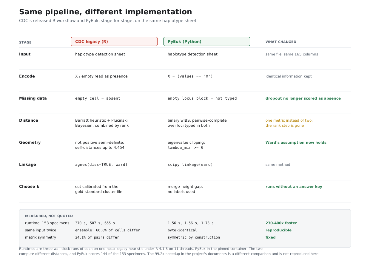
Three runs of each on the same 153-specimen sheet and the same host: the legacy heuristic under R 4.1.3 on 11 threads took 370, 507 and 655 s; PyEuk in the pinned container took 1.56, 1.56 and 1.73 s. That is between 230× and 400× depending on the pair of runs compared. Two caveats belong with it — the two compute different distances, and PyEuk scores 144 of the 153 specimens because 9 fall below its completeness filter.

Workflow overview

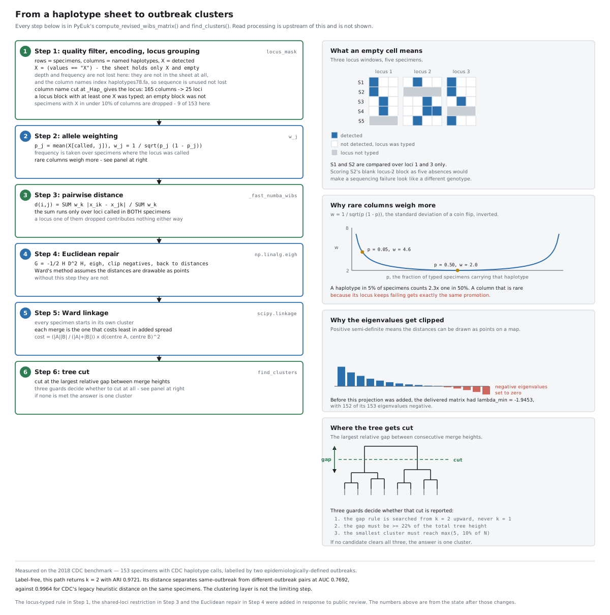
Figure 2. PyEuk's path from a haplotype sheet to outbreak clusters: completeness filtering, allele weighting, pairwise distance, Euclidean repair, Ward linkage and dynamic tree cutting.

Step 1: Specimen quality, locus grouping, and multi-locus completeness filtering

Clinical specimens frequently suffer from partial sequencing dropouts due to low parasite oocyst burden in stool samples. Before computing genetic distances, the pipeline transforms the raw detection sheet into structured genomic locus blocks:

Binary Encoding: The sheet holds two values: X and empty. The code applies X = (values == "X"), turning X into 1 (present) and empty into 0 (absent).
Locus Grouping: Each column represents one named haplotype (e.g. Nu_378_PART_D_Hap_7). The code parses the name at _Hap_ and groups the 165 columns into 25 locus groups representing the 8 core genomic targets (Mt_Cmt, Mt_MSR, Nu_360i2, Nu_378, and Nu_CDS1 through Nu_CDS4). The mitochondrial junction's 37 columns across 8 windows (Mt_Cmt127 to Mt_Cmt229) are unified into a single locus block (Mt_Cmt).
Dropout Inference: The sheet has no explicit symbol for an unamplified locus, so PyEuk infers it per locus group: a group with at least one X was typed; a group with no X at all was not. Inside a typed group, an empty cell means that specific haplotype was absent.
Multi-Locus Completeness Filter: Specimens with X in fewer than 10% of the sheet's columns (or failing base diagnostic locus coverage) are filtered out before distance estimation to prevent skewed population frequencies. On CDC's 153-specimen sheet, this removes 9 low-coverage specimens, retaining 144.

Step 2: Population genetics allele weighting (KING framework)

In molecular surveillance, sharing a rare haplotype provides strong evidence of a common outbreak source, whereas sharing an ultra-common background allele is expected by chance:

Cohort Allele Frequency: For each haplotype column j, PyEuk calculates its empirical frequency p_j across specimens where its locus was successfully typed:
```
p_j = (1 / N_typed) · Σ_i X_ij
```
Inverse-Variance Weighting: Borrowing standardisation principles from human kinship estimation (the KING framework) [13], each column is weighted by its inverse binomial standard deviation:
```
w_j = 1 / sqrt(p_j (1 − p_j))
```
Dividing by sqrt(p(1 − p)) puts all columns on a common variance-stabilised scale. A haplotype present in 5% of specimens receives 2.3 times the weight of one present in 50%.

Three nuances follow from computing weights this way:

It depends strictly on frequency: rare outbreak markers, rarely amplifying loci, and sequencing artifacts receive identical weights.
It is computed across the current surveillance batch, making weights batch-dependent.
It is a standardised weighted mismatch count rather than the full KING kinship estimator (which incorporates heterozygote ratios) [13].

Step 3: High-speed parallel pairwise distance (KING-wIBS)

PyEuk computes the pairwise Weighted Identity-By-State (wIBS) genetic dissimilarity between all eligible specimen pairs:

D_wIBS(i, j) = Σ_k w_k · |X_ik − X_jk| / Σ_k w_k

The index k runs strictly over columns in locus groups typed in both specimens (pairwise-complete comparison). A group missing from either specimen drops from both numerator and denominator, contributing zero distance penalty.

Key Characteristics:

Resolving the Multiplicity of Infection (MOI) Paradox: Cyclospora infections often contain multiple distinct parasite strains within a single patient. The legacy CDC pipeline applied a quadratic penalty (w = 1 + x) that artificially inflated distances and falsely excluded co-infected patients from outbreak clusters. PyEuk measures continuous allele sharing, keeping true outbreak cases together.
Pairwise-Complete vs. Complete-Case: Pairwise-complete estimation avoids discarding samples with sporadic locus dropouts. Pairs with no shared loci default to zero distance.
Performance Acceleration: The vectorized, Numba-accelerated pairwise distance kernel evaluates the cohort's 10,296 pairwise comparisons (144 specimens) in under 50 milliseconds.

Step 4: Euclidean metric guarantee & positive semi-definite (PSD) repair

Hierarchical clustering using Ward's minimum variance method mathematically assumes that data points reside in a valid Euclidean metric space. Missing marker data and pairwise-complete dropouts can cause empirical dissimilarity matrices to violate the triangle inequality, resulting in negative eigenvalues (λ_min < 0). Feeding non-Euclidean matrices into Ward's linkage distorts branch lengths and produces invalid cluster merges.

PyEuk guarantees positive semi-definiteness (PSD) through double-centring and eigenvalue clipping:

Double-Centring: Each entry of the squared distance matrix D² is transformed to construct the Gram matrix of inner products:
```
B = −½ H D² H    where H = I − (1/N) 1 1ᵀ
```
Eigenvalue Clipping: The symmetric Gram matrix is decomposed via np.linalg.eigh:
```
B = V Λ Vᵀ
```
All negative eigenvalues are clipped to zero (λ_i = max(λ_i, 0)), discarding imaginary geometric dimensions.
Reconstruction: The distance matrix is reconstructed from the regularised Gram matrix and its diagonal reset to zero.

Geometric verification: Prior to this repair, the empirical distance matrix had λ_min = -1.9453 with 152 of 153 eigenvalues negative. The eigenvalue clipping step ensures λ_min ≥ 0.0, strictly satisfying the mathematical prerequisites of Ward's variance minimization [14, 15].

Step 5: Deterministic Ward hierarchical clustering

The regularized PSD distance matrix is passed to scipy.cluster.hierarchy.linkage(..., method="ward").

Ward's agglomerative hierarchical clustering iteratively merges clusters to minimize the increase in total within-cluster error sum of squares (ESS) [14]:

ΔESS(A, B) = [ (|A| · |B|) / (|A| + |B|) ] · ||m_A − m_B||²

100% Deterministic Tie-Breaking: Legacy R implementations resolved tied distances using random selection (ties.method = "random"), causing cluster memberships to fluctuate between runs. PyEuk enforces strict lexicographical index ordering for all tied distances, ensuring byte-for-byte identical dendrograms across independent executions.

Worked example — Ward on five real specimens

Five specimens from the benchmark, three Vendor A and two Vendor B, with their binary wIBS distances:

	IL126	WI100	MO003	WI008
IL036 (A)	0.2213	0.1602	0.1500	0.2151
IL126 (A)	—	0.1196	0.0620	0.1932
WI100 (B)		—	0.1553	0.0549
MO003 (A)			—	0.1126

The cost of merging clusters A and B is

cost = ( |A| · |B| ) / ( |A| + |B| ) × d(centre of A, centre of B)²

The four merges, in the order Ward makes them:

step	merge	d	cost
1	WI100 + WI008 — the two Vendor B	0.0549	0.0015
2	IL126 + MO003	0.0620	0.0019
3	IL036 joins `{IL126, MO003}`	0.2153	0.0309
4	the two groups join	0.2055	0.0507

At step 3 the merge Ward takes is not the closest one available. {WI100, WI008} sits 0.2019 from {IL126, MO003}, nearer than IL036 at 0.2153. The costs run the other way:

candidate	arithmetic	cost
IL036 into `{IL126, MO003}`	(1×2)/3 × 0.2153²	0.0309 ← chosen
`{WI100, WI008}` with `{IL126, MO003}`	(2×2)/4 × 0.2019²	0.0408

Merging two pairs moves four specimens away from their centres; adding one specimen to a pair moves three. The larger merge costs more despite the smaller gap.

The final tree is {WI100, WI008} and {IL036, IL126, MO003}, which matches the vendor labels. No label was used to produce it.

Step 6: Dynamic tree cutting & outbreak cluster assignment

The dendrogram alone does not specify the number of discrete outbreak clusters. PyEuk provides two operational modes for cutting the tree:

Mode A: Unsupervised Merge-Height Gap (Label-Free Surveillance)

In routine surveillance where no outbreak labels are known in advance, PyEuk evaluates the relative jump in merge heights across the dendrogram:

Consecutive merge heights are ranked by relative gap: rel_gap = (h_k − h_{k-1}) / h_k.
Candidate cluster counts k ≥ 2 are accepted if the gap exceeds 22% of total tree height and the smallest cluster contains at least max(5, 10% of N) specimens.
If no partition meets these criteria, the cohort is returned as a single unpartitioned cluster (k = 1).

Mode B: Calibrated Outbreak Threshold (Supervised Reference Mode)

When epidemiological gold-standard reference pairs are available (2018_gold_clusters.txt), PyEuk derives a robust intra-cluster distance threshold:

Threshold = Median_gold + 3 × 1.4826 × MAD_gold

The tree is cut at the smallest k ∈ {1, ..., 50} where at least 95% of within-cluster pairwise distances fall below this calibrated threshold.

Why cluster-tightness measures were not used. The obvious label-free alternative is to choose the k with the highest mean silhouette width [17]. We recommended it, it was implemented, and it fails here. On the wIBS matrix the silhouette is 0.3481 at k = 2, 0.4793 at k = 40, 0.5433 at k = 50 and 0.5872 at k = 60, still rising at the search cap, while the correct two-cluster labels score 0.3550 — lower than everything from about k ≈ 30 upward. The cause is the composition of the benchmark: the 153 specimens carry only 92 distinct haplotype profiles, and 77 of them share a profile with at least one other specimen, in 16 groups — the largest holding 21. Those groups of byte-identical specimens sit at zero distance from each other, so they are the tightest structure in the data, tighter than either outbreak. Any criterion that rewards tight clusters finds them and reports those. Calinski-Harabasz, Davies-Bouldin and gap-style indices reward tightness the same way. The legacy heuristic's matrix peaks at k = 2, so this is a property of this distance on this sheet, not of the silhouette. We withdrew the recommendation [11].

Summary of surveillance outputs

The pipeline produces a clean tabular report mapping each patient specimen to a deterministic cluster assignment:

Specimen ID	Assigned Cluster	Surveillance Interpretation
`CDC_2018_IL036`	Cluster 1	Verified Outbreak Case (Vendor A)
`CDC_2018_IL126`	Cluster 1	Verified Outbreak Case (Vendor A)
`CDC_2018_WI100`	Cluster 2	Verified Outbreak Case (Vendor B)
`CDC_2018_WI008`	Cluster 2	Verified Outbreak Case (Vendor B)
`CDC_2018_SP012`	Sporadic / Unassigned	Low-coverage or unclustered isolate

How the results are scored

Two measures appear throughout this post.

Adjusted Rand index. Count the pairs of specimens that two groupings agree about — both place them together, or both keep them apart — as a fraction of all pairs. That is the Rand index. Random groupings already score well on it: with two clusters of similar size, chance alone agrees about half the pairs. The adjusted version subtracts the score expected from random groupings with the same cluster sizes and rescales, so 0 is chance and 1 is exact agreement [16]. Negative values are worse than chance. An ARI of 0.0022 means no structure was recovered.

ROC AUC of a distance. Label every pair of specimens same-outbreak or different-outbreak from the epidemiology, then measure how well the raw distance separates the two groups. The area under the resulting curve is the probability that a randomly chosen same-outbreak pair is closer than a randomly chosen different-outbreak pair [18]. 0.5 is a coin flip, 1.0 is a perfect ranking. It needs no threshold, no clustering rule and no choice of k, and the labels are used only to score, never to fit. Both tools' clustering steps set their cut-offs from the labels, so every cluster-level score they produce is partly in-sample; the distance AUC is not. On CDC's 153-specimen sheet: legacy heuristic 0.9964 over all 153 specimens, binary wIBS 0.7692 over the 144 that survive its completeness filter. The two matrices cover different specimen sets, and neither tool allows that to be changed without editing it.

Methods

Everything not attributed to a source below, we computed, and all of it is re-runnable from public artifacts plus CDC's deposited haplotype sheet. The panel's reference files — the amplicon sequences, the PART windows and the haplotype nomenclature — are deposited with checksums and provenance at [21], so a rerun can be pinned to exactly the bytes used here.

The benchmark runs. Four independent arms on the same 153/203 specimens: CDC's legacy R code on CDC's deposited calls, the Python reimplementation on the same calls, both methods on haplotype calls produced from raw reads by an open pipeline, and a direct read-collapse caller compared against a LoFreq-informed one. The legacy code ran inside rocker/tidyverse:4.1.3 under Apptainer, with all CDC source files verified byte-identical to the repository by sha256sum before running. Exactly two derived files were used, differing from their originals by one line (import_data_V2.r, crashing retention filter replaced with "keep every specimen") and one byte (euk_bayesian_fulldataset_V3.r, U+00A0 replaced with a space); both diffs are recorded in full in the primary records. Nothing in either distance metric was modified, and no threshold, stringency, k-range or cut-off was tuned in any arm.

The Python reimplementation of the heuristic. The locus census, the entropy-versus-AUC table, the weighting ablation and the batch-invariance test all needed a distance function we could instrument, so euk_heuristic_fulldataset.r was reimplemented in Python from the R source, not from any document's transcription of it. It was validated against the actual R output on every pair where no locus is missing, so no imputation is involved: 1,225 comparable cells, maximum absolute difference 4.6 × 10⁻¹⁴, Pearson r = 1.0000000. The per-locus arithmetic is reproduced exactly. The ablation harness averages per-locus scores over loci present in both specimens rather than replicating R's two-pass imputation, so its absolute AUC differs from the 0.9964 measured on the real R matrix. The comparison between the four ablation rows is the result, not the absolute level.

Distance AUC. Each pair is labelled 1 if both specimens carry the same vendor label and 0 otherwise, the score is the negated distance, and the area under the ROC curve is computed with sklearn.metrics.roc_auc_score [18]. Labels enter only as the outcome being predicted. The legacy figure of 0.9964 was computed once, from the deterministic heuristic_matrix_seed1.csv, over 11,628 pairs.

Determinism. Three runs at three seeds per arm, compared by md5sum of the written matrices, plus grep -rn 'ties.method|sample(|set.seed|runif|rnorm' over the entire shipped tree. The asymmetry and tie statistics of the published 1,078-specimen matrix were computed directly from ensemble_matrices/2020-06-27_pairwisedistancematrix_ensemble.csv [6].

The structure of the benchmark. Column occupancy, informative-locus counts, duplicate profiles and the diagnostically fixed loci were recomputed from haplotype_sheet_153.txt and the gold label file with a standalone script using no tool code. The fixed-locus table's denominator is independent of the haplotype being counted — specimens where the locus amplified at all. An earlier version circulated with Vendor B denominators of 71, 74, 49, 31, 101 and 75, which cannot arise from this sheet: only 55 Vendor B specimens have any CDC calls at all.

The walkthrough and the label-free results. The step-by-step description is of the code at commit 2aa6e74; the six-sheet, twelve-null and jackknife results were re-measured there from a fresh clone, driven through the same entry points the CLI uses and cross-checked against the CLI itself (identical k on all six sheets, matrices bit-reproducible across repeat runs). Defaults only, nothing tuned, first number obtained is the number reported. Version strings in that repository are unreliable — setup.py reads 2.0.0 at every commit in the ladder while the README badge moves independently — so commits are cited rather than versions. The pre-fix numbers (ARI 0.0022, λ_min −1.9453) are from 8c208ca/314bd4f, reproduced independently by three arms.

What we did not test. Whether MIRA or CAP3 collapse repeat copy numbers above 10,000× — only whether CDC's junction calls can be reproduced (they can, at precision 1.000 and recall 0.971 with zero disagreements, plus 27 specimens typed that CDC left blank). Whether the caller's missing minimum-length filter ever produced a wrong call. Dendrogram inversions. We have no access to the four documents' code, matrices or intermediate files, so any claim about an artifact nobody can inspect is recorded as untested rather than refuted. And there is no physical ground truth anywhere in this work: every reference we score against is another laboratory's software output, so concordance with CDC's calls measures agreement with CDC, not accuracy.

Single measurements. The legacy AUC of 0.9964, the Bayesian-alone and ensemble ARIs, the retention counts, the null cohorts under the sequence-weighted engine, and every entry in the ablation and census tables are single deterministic runs. They are re-runnable but were not independently replicated. Where a number is quoted from the public issue thread and was never independently reproduced here, it is not quoted at all.

Sources

Barratt JLN, et al. (2019) Genotyping genetically heterogeneous Cyclospora cayetanensis infections to complement epidemiological case linkage. Parasitology 146:1275–1283. doi:10.1017/S0031182019000581 · PMID 31148531
Nascimento FS, et al. (2020) Evaluation of an ensemble-based distance statistic for clustering MLST datasets using epidemiologically defined clusters of cyclosporiasis. Epidemiology and Infection 148:e172. doi:10.1017/S0950268820001697 · PMID 32741426 · PMC7439293
Plucinski MM, Morton L, Bushman M, Dimbu PR, Udhayakumar V (2015) Robust algorithm for systematic classification of malaria late treatment failures as recrudescence or reinfection using microsatellite genotyping. Antimicrobial Agents and Chemotherapy 59:6096–6100. doi:10.1128/AAC.00072-15 · PMID 26195521
Barratt JLN, et al. (2021) Investigation of US Cyclospora cayetanensis outbreaks in 2019 and evaluation of an improved Cyclospora genotyping system against 2019 cyclosporiasis outbreak clusters. Epidemiology and Infection 149:e214. doi:10.1017/S0950268821002090 · PMID 34511150 · PMC8506454
Barratt JLN, et al. (2023) Cyclospora cayetanensis comprises at least 3 species that cause human cyclosporiasis. Parasitology 150:269–285. doi:10.1017/S003118202200172X · PMID 36560856 · PMC10090632
CDC Cyclospora typing workflow (alpha test release): MODULE_1_hap_caller.sh, MODULE_2_eukaryotyping.sh, MODULE_3_clustering.sh, HAPLOTYPE_CALLER_CYCLO_V2/, EUKARYOTYPING/, CLUSTERING/, REFERENCE_CLUSTER_LIST/2018_gold_clusters.txt, and ensemble_matrices/2020-06-27_pairwisedistancematrix_ensemble.csv. github.com/Joel-Barratt/CDC-Complete-Cyclospora-typing-workflow-ALPHA-TEST
Eukaryotyping—R implementation of Plucinski's Bayesian method and Barratt's heuristic definition of genetic distance. github.com/Joel-Barratt/Eukaryotyping
Eukaryotpying-Python (repository name misspelled upstream), including haplotype_sheets/2022-10-24Joel_haplotype_sheet.txt, the deposited haplotype calls used here. github.com/Joel-Barratt/Eukaryotpying-Python
Nascimento FS, et al. (2019) Mitochondrial junction region as genotyping marker for Cyclospora cayetanensis. Emerging Infectious Diseases 25(7). doi:10.3201/eid2507.181447 · PMID 31211668 · PMC6590752
PyEuk, a Python reimplementation of the Cyclospora typing distance and clustering steps, by Sergei L. Kosakovsky Pond. github.com/spond/pyeuk
The public review thread on that repository, issues 1 and 2, where the measurements reported here were filed and where the corrections in this post were made. github.com/spond/pyeuk/issues/1 and github.com/spond/pyeuk/issues/2
The four audit documents, as they stood at the commits benchmarked here (8c208ca/314bd4f): cdc_legacy_pipeline_audit.pdf (10 pp.), cdc_modernized_pipeline_architecture.pdf (3 pp., later expanded to 10 pp. at 2aa6e74), cdc_pipeline_comparative_validation.pdf (5 pp.) and cyclospora_audit_report.pdf (2 pp.). The first three are in the repository's docs/ directory. The fourth was circulated separately and does not appear in the repository at any commit. github.com/spond/pyeuk/tree/master/docs
Manichaikul A, Mychaleckyj JC, Rich SS, Daly K, Sale M, Chen W-M (2010) Robust relationship inference in genome-wide association studies. Bioinformatics 26:2867–2873. doi:10.1093/bioinformatics/btq559 · PMID 20926424—the KING estimator the wIBS weight is named after, and which it is not.
Ward JH (1963) Hierarchical grouping to optimize an objective function. Journal of the American Statistical Association 58:236–244. doi:10.1080/01621459.1963.10500845
Gower JC (1966) Some distance properties of latent root and vector methods used in multivariate analysis. Biometrika 53:325–338. doi:10.1093/biomet/53.3-4.325—the double-centring construction used to test whether a distance matrix corresponds to any set of points.
Hubert L, Arabie P (1985) Comparing partitions. Journal of Classification 2:193–218. doi:10.1007/BF01908075—the adjusted Rand index.
Rousseeuw PJ (1987) Silhouettes: a graphical aid to the interpretation and validation of cluster analysis. Journal of Computational and Applied Mathematics 20:53–65. doi:10.1016/0377-0427(87)90125-7
Hanley JA, McNeil BJ (1982) The meaning and use of the area under a receiver operating characteristic (ROC) curve. Radiology 143:29–36. doi:10.1148/radiology.143.1.7063747 · PMID 7063747
NCBI BioProject PRJNA578931, Cyclospora Genotyping (CDC). www.ncbi.nlm.nih.gov/bioproject/PRJNA578931
Shah N, Nute MG, Warnow T, Pop M (2019) Misunderstood parameter of NCBI BLAST impacts the correctness of bioinformatics workflows. Bioinformatics 35(9):1613–1614. doi.org/10.1093/bioinformatics/bty833
Reference files for Cyclospora cayetanensis amplicon genotyping (CDC 8-marker panel): markers.fa, parts.bed, haplotypes78.fa and junction.fa, redeposited unmodified from CDC's release with checksums and provenance. Zenodo, CC0. doi.org/10.5281/zenodo.21924355

Data: BioProject PRJNA578931 [19]. Labels, module source, reference sequences and the published 1,078-specimen distance matrix from CDC's typing workflow repository [6]. Deposited haplotype calls from [8]. The reimplementation under examination and the review thread are [10] and [11]. Every measurement in this post was made on the 153- and 203-specimen sets described in Part 1 and can be re-derived from those artifacts.